
Amodeo (JMP, 2025)
This paper studies the impact of interest rate disagreement between the Federal Reserve and financial markets on the transmission of U.S. monetary policy. First, I construct a simple real-time measure of disagreement and show that it improves short- and medium-horizon forecasts in standard macroeconomic VARs. Second, using lag-augmented local projections, I show that disagreement dampens monetary policy effectiveness, attenuating its impact on output and offering an explanation for apparent anomalies such as the 'activity puzzle.' Third, I demonstrate that market expectations, as reflected in tradable asset prices, outperform Fed staff forecasts, and that information-advantage tests reveal no systematic Fed edge, challenging prevailing narratives. I show that standard New Keynesian frameworks with incomplete information contain a latent disagreement structure, which, when formalized, yields a parsimonious explanation of the documented evidence. The model generates disagreement from three distinct sources — fundamentals, policy rule, and credibility. A general state-space model identifies the importance of each and sheds light on key normative implications.
Methodology
Amodeo (JMP, 2025)
This paper studies the impact of interest rate disagreement between the Federal Reserve and financial markets on the transmission of U.S. monetary policy. First, I construct a simple real-time measure of disagreement and show that it improves short- and medium-horizon forecasts in standard macroeconomic VARs. Second, using lag-augmented local projections, I show that disagreement dampens monetary policy effectiveness, attenuating its impact on output and offering an explanation for apparent anomalies such as the 'activity puzzle.' Third, I demonstrate that market expectations, as reflected in tradable asset prices, outperform Fed staff forecasts, and that information-advantage tests reveal no systematic Fed edge, challenging prevailing narratives. I show that standard New Keynesian frameworks with incomplete information contain a latent disagreement structure, which, when formalized, yields a parsimonious explanation of the documented evidence. The model generates disagreement from three distinct sources — fundamentals, policy rule, and credibility. A general state-space model identifies the importance of each and sheds light on key normative implications.
Amodeo (JMP, 2025)
"This paper studies the impact of interest rate disagreement between the Federal Reserve and financial markets on the transmission of U.S. monetary policy. First, I construct a simple real-time measure of disagreement and show that it improves short- and medium-horizon forecasts in standard macroeconomic VARs. Second, using lag-augmented local projections, I show that disagreement dampens monetary policy effectiveness, attenuating its impact on output and offering an explanation for apparent anomalies such as the 'activity puzzle.' Third, I demonstrate that market expectations, as reflected in tradable asset prices, outperform Fed staff forecasts, and that information-advantage tests reveal no systematic Fed edge, challenging prevailing narratives. I show that standard New Keynesian frameworks with incomplete information contain a latent disagreement structure, which, when formalized, yields a parsimonious explanation of the documented evidence. The model generates disagreement from three distinct sources — fundamentals, policy rule, and credibility. A general state-space model identifies the importance of each and sheds light on key normative implications."
m = 60 is unavailable because the reduced sample leaves too few observations to evaluate the test window.
m = 60 is unavailable because the reduced sample leaves too few observations to evaluate the test window.
Amodeo (JMP, 2025)
"This paper studies the impact of interest rate disagreement between the Federal Reserve and financial markets on the transmission of U.S. monetary policy. First, I construct a simple real-time measure of disagreement and show that it improves short- and medium-horizon forecasts in standard macroeconomic VARs. Second, using lag-augmented local projections, I show that disagreement dampens monetary policy effectiveness, attenuating its impact on output and offering an explanation for apparent anomalies such as the 'activity puzzle.' Third, I demonstrate that market expectations, as reflected in tradable asset prices, outperform Fed staff forecasts, and that information-advantage tests reveal no systematic Fed edge, challenging prevailing narratives. I show that standard New Keynesian frameworks with incomplete information contain a latent disagreement structure, which, when formalized, yields a parsimonious explanation of the documented evidence. The model generates disagreement from three distinct sources — fundamentals, policy rule, and credibility. A general state-space model identifies the importance of each and sheds light on key normative implications."
Title Customization
Overall Graph Font
This font applies to graph title, axis labels, and tick labels when not overridden by specific settings.
Federal Funds Rate
Taylor Rule
Market Forecasts (Day After FOMC)
Market Forecasts (Day Before FOMC)
Greenbook/Fed Forecasts
Legend Settings
Configure the mathematical formula display that shows the current Taylor Rule equation.
Background & Colors
Configure the appearance of historical "ghost" lines in stop motion mode.
Taylor Rule Ghost Lines
Greenbook Ghost Lines
Market Ghost Lines
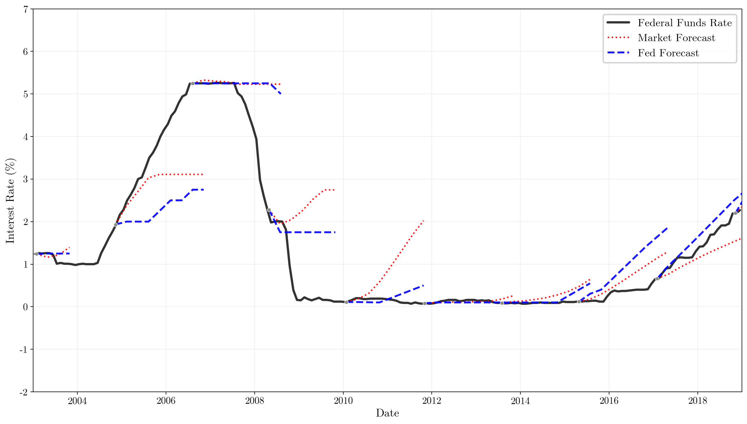
Figure 1. Black solid line —effective federal funds rate. Red dashed — meeting-day market-implied expectations from federal funds futures. Blue dashed — Fed policy-rate expectations from the Tealbook.
3.4 Predictive Accuracy
Table 3. Diebold–Mariano tests of equal predictive accuracy (Market vs Fed) across horizons with Market’s forecast on the day of the Tealbook (internal) release. Reported are sample size \(N\), test statistic, \(p\)-value, and the lower-MSE winner.
3.1 Disagreement About Monetary Policy
I define disagreement as the Tealbook minus futures path for the federal funds rate, document its slow-moving yet weakly countercyclical behavior via the moments in Table 1, and chart its evolution since 1988 in Figure 5.
For each forecast horizon \(h\), define disagreement
where \(i_{t+h}\) denotes the federal funds rate \(h\) quarters ahead, \(E_t^F\) is the Fed’s expectation (from the Greenbook/Tealbook) and \(E_t^M\) is the market’s expectation (implied from traded futures). Note that by construction (1) is signed and order-sensitive—swapping Fed and Market flips the sign; in some of the exercises I will use its absolute value.
As a summary of differences between Fed and market expectations, I compute average disagreement simply as the arithmetic mean over the available horizons of \(D_t^h\). Table 1 summarizes moments and regime means. Disagreement is slow-moving and highly persistent, with a positive tilt — the Fed’s path exceeds markets in about 47% of months. Mean absolute disagreement is higher in recessions than in expansions, but the recession–expansion gap is imprecisely estimated and not statistically significant. Overall, disagreement is at most weakly countercyclical in magnitude and shows negligible cyclicality in sign.
Figure 5 plots the time series of the average \(D_t^h\) over all available horizons throughout 1988:10–2019:12, with NBER-dated recessions shaded.
Panel A. Unconditional moments.
| Mean | SD | AR(1) | Pr > 0 | |
|---|---|---|---|---|
| \( \overline{D}_t \) | 0.058 | 0.490 | 0.925 | 0.465 |
| \( |\overline{D}_t| \) | 0.383 | 0.310 | 0.866 | 1.000 |
Panel B. Means by business-cycle regime.
| Exp. \( N = 333 \) | Rec. \( N = 37 \) | Rec–Exp | p-val | |
|---|---|---|---|---|
| \( \overline{D}_t \) | 0.065 | -0.005 | -0.069 | 0.734 |
| \( |\overline{D}_t| \) | 0.375 | 0.454 | 0.079 | 0.275 |
Table 1. Disagreement: Unconditional Moments and Business-Cycle Means. Notes: Monthly data, 1988:10–2019:12. Units: percentage points. “Rec–Exp” and \(p\)-values from Newey–West regressions with 12 lags. \(\overline{D}_t\) is the unweighted mean of \(D_t^h = E_t^F(i_{t+h}) - E_t^M(i_{t+h})\); \(|\overline{D}_t|\) is its absolute value. NBER recession dates.
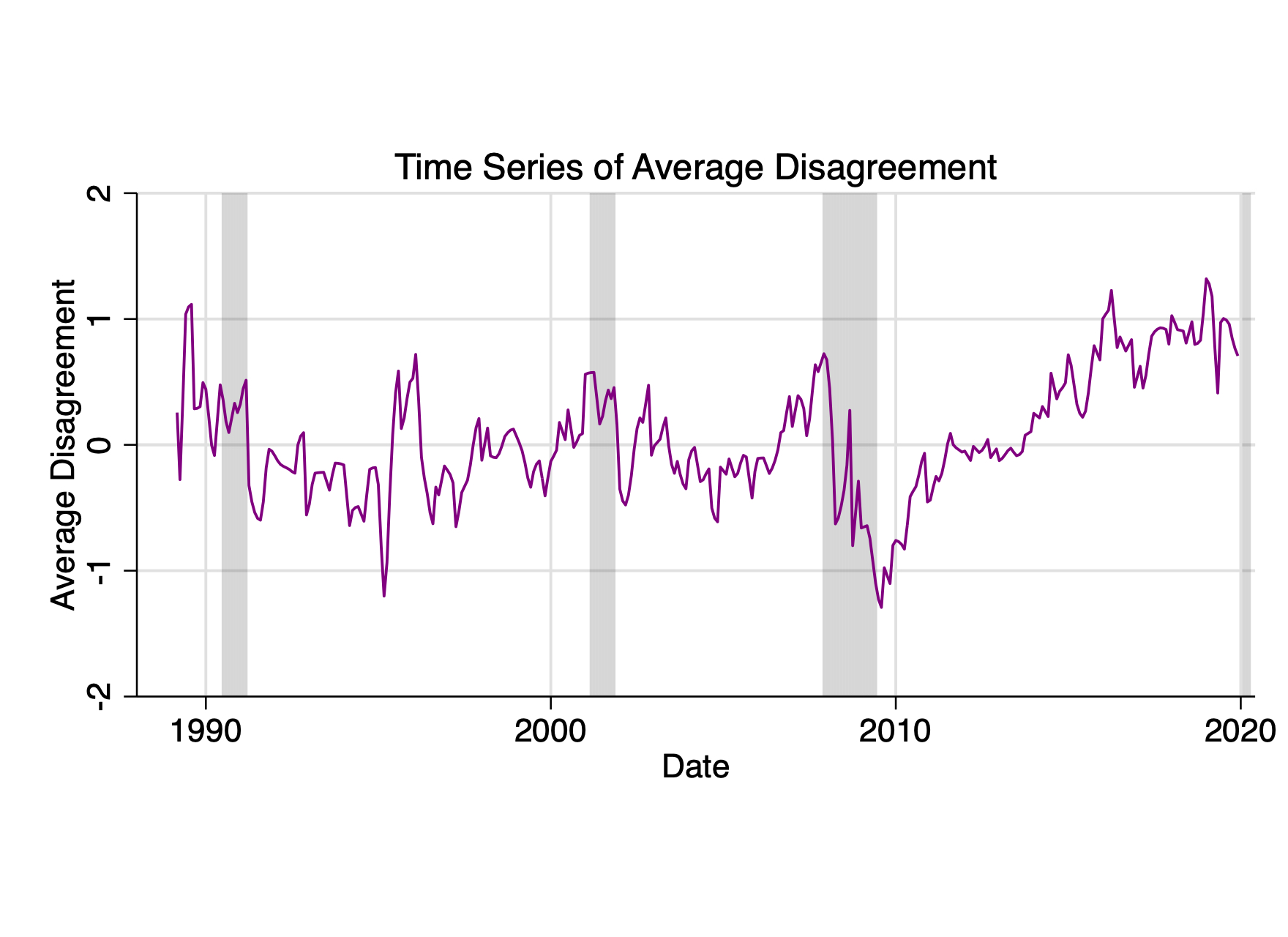
Figure 5. Fed–Market Average Disagreement. Quarterly frequency. Sample: 1988:10–2019:12. Shaded gray areas correspond to NBER recession dates.
3.2 Predictive Power of Disagreement
I feed the disagreement measure into standard IP–CPI–FFR VARs and block-Granger tests reject the no-predictive-power null through roughly six quarters, implying meaningful forecast-error reductions for output, inflation, and policy.
Disagreement between markets’ and the Fed’s expectations is pervasive and likely reflects differential views on fundamentals, policy rules, or future behavior of the FOMC. These frequent divergences allow me to construct a measure of disagreement that may carry information for future macroeconomic outcomes. This section shows that such a measure is indeed helpful in forecasting exercises in commonly specified macroeconomic vector autoregressions.
I estimate VARs with three variables — industrial production, consumer prices, and the policy rate — and perform block Granger causality tests to establish whether the newly obtained disagreement variable statistically improves the forecasting of any of the specified variables. The null hypothesis \(H_{0}\) is that all lag coefficients on \(D^{h}_{t}, \ldots, D^{h}_{t-p}\) are zero. Rejection implies that \(p\) lags of \(D^{h}_{t}\) improve conditional forecasts of \([\mathrm{IP}_{t}, \pi_{t}, i_{t}]\).
Table 2 reports block F-statistics for horizons of one to eight quarters. The null that disagreement (and its lags) does not Granger-cause macroeconomic aggregates is rejected at the 5% significance level across these horizons. At horizons seven and eight quarters the F-statistics fall and the null cannot be rejected, indicating that the predictive power of disagreement weakly fades beyond about a year and a half.
More precisely, adding \(D^{h}_{t}\) yields non-trivial relative gains. Measured as the percent drop in unexplained variance, for \(i_{t}\) it peaks near 15–16% at \(h = 5\text{--}6\); for \(\pi_{t}\) about 9–13% at \(h = 5\text{--}8\); for \(\mathrm{IP}_{t}\) about 4–8% at \(h = 3\text{--}6\). This aligns with the block-Granger rejections8.
| Null: \(H_{0}\) | Distribution | Statistic | PValue | Decision |
|---|---|---|---|---|
| Exclude \(\{D^{1}_{t,\ldots,t-p}\}\) | F(21,335) | 2.468 | 0.000 | Reject |
| Exclude \(\{D^{2}_{t,\ldots,t-p}\}\) | F(18,340) | 2.261 | 0.003 | Reject |
| Exclude \(\{D^{3}_{t,\ldots,t-p}\}\) | F(24,305) | 2.224 | 0.001 | Reject |
| Exclude \(\{D^{4}_{t,\ldots,t-p}\}\) | F(18,255) | 2.852 | 0.000 | Reject |
| Exclude \(\{D^{5}_{t,\ldots,t-p}\}\) | F(30,148) | 2.065 | 0.002 | Reject |
| Exclude \(\{D^{6}_{t,\ldots,t-p}\}\) | F(30,141) | 1.960 | 0.005 | Reject |
| Exclude \(\{D^{7}_{t,\ldots,t-p}\}\) | F(30,141) | 1.417 | 0.092 | Fail to Reject |
| Exclude \(\{D^{8}_{t,\ldots,t-p}\}\) | F(27,139) | 1.315 | 0.156 | Fail to Reject |
| Exclude \(\{\overline{D}_{t,\ldots,t-p}\}\) | F(18,340) | 2.308 | 0.002 | Reject |
Table 2. Block Granger Causality: 1–8 quarters and average; Null \(H_{0} : \Phi_{n,1,p} = 0\ \forall p\) (no predictive power) at \(\alpha = 0.05\) significance level. Based on an estimated VAR with a constant including \([\mathrm{FFR}_{t}, D_{t}, \mathrm{CPI}_{t}, \mathrm{IP}_{t}]\), where \(D_{t}\) is either a vintage \(D^{h}_{t}\) or the summary measure \(\bar D_{t}\). Number of lags is picked by the most conservative between the Akaike and Schwartz criteria \((p = \max(\mathrm{AIC}, \mathrm{SBC}))\). See Appendix C for further estimation details.
3.4.1 Revisiting Fed's Informational Advantage
Quarter-by-quarter forecast informational advantage test figures showing Federal Funds Rate Forecasts for Q1 through Q8.
Federal Funds Rate, Q1
Federal Funds Rate, Q2
Federal Funds Rate, Q3
Federal Funds Rate, Q4
Federal Funds Rate, Q5
Federal Funds Rate, Q6
Federal Funds Rate, Q7
Federal Funds Rate, Q8
Amodeo (JMP, 2025)
"This paper studies the impact of interest rate disagreement between the Federal Reserve and financial markets on the transmission of U.S. monetary policy. First, I construct a simple real-time measure of disagreement and show that it improves short- and medium-horizon forecasts in standard macroeconomic VARs. Second, using lag-augmented local projections, I show that disagreement dampens monetary policy effectiveness, attenuating its impact on output and offering an explanation for apparent anomalies such as the 'activity puzzle.' Third, I demonstrate that market expectations, as reflected in tradable asset prices, outperform Fed staff forecasts, and that information-advantage tests reveal no systematic Fed edge, challenging prevailing narratives. I show that standard New Keynesian frameworks with incomplete information contain a latent disagreement structure, which, when formalized, yields a parsimonious explanation of the documented evidence. The model generates disagreement from three distinct sources — fundamentals, policy rule, and credibility. A general state-space model identifies the importance of each and sheds light on key normative implications."
3.3 Disagreement and the Transmission of Monetary Policy
3.3.1 Disagreement and Uncertainty
Exploring the relationship between disagreement and uncertainty in monetary policy transmission.
To isolate disagreement from broader volatility forces, we augment equation (3) with VIX- and SPF-based uncertainty interactions so the attenuation in monetary transmission remains robust to both financial and macro risk conditions.
Two identification threats are central: cyclical comovement and uncertainty. Disagreement may rise in weak times or during risk spikes, and it may respond to the volatility of the economic environment. In fact, disagreement's endogeneity might invalidate the causal interpretation of the estimates from the regressions in (2).
While the conservative lag-specification allows for a robust control of the state of the economy, disagreement seems inherently related to the uncertainty in the economic environment. A more uncertain or volatile outlook might imply more uncertain or volatile forecasts, which can widen the gap in expectations between the Fed and financial markets. Although there is a weak negative unconditional correlation between the measures of uncertainty I employ and the absolute average disagreement measure13, I address this by augmenting equation (2) in two separate ways: (i) including the VIX index (and its lags) interacted with the monetary policy shock in the regressions, controlling for financial uncertainty; (ii) including the cross-sectional dispersion of the responses to the Survey of Professional Forecasters (and its lags) also interacted with the monetary policy surprises, controlling for macro uncertainty14.
Let $\upsilon_t = \left(VIX_t, SPF_t\right)$15:
with $\text{Lags}_{t-1}^L\equiv\big[\,\mathbf{y}_{t-1:t-L},\; s_{t-1:t-L},\; v_{t-1:t-L}\,\big]^{\prime}$ and $\boldsymbol{\theta}_h\equiv[\,\phi_{h}^{1:L},\ \gamma_{h}^{1:L},\ \zeta_{h}^{1:L}\,]$.
As Figure 9 shows for $\upsilon_t = VIX_t$, the marginal effect of disagreement (right panel) is left practically intact, while $\alpha_h$ – the response of industrial production to a monetary shock in the absence of disagreement and uncertainty – is accentuated. This finding suggests that the attenuation associated with the level of disagreement in the economy is robust to the inclusion of a widely used index of economic uncertainty and volatility.
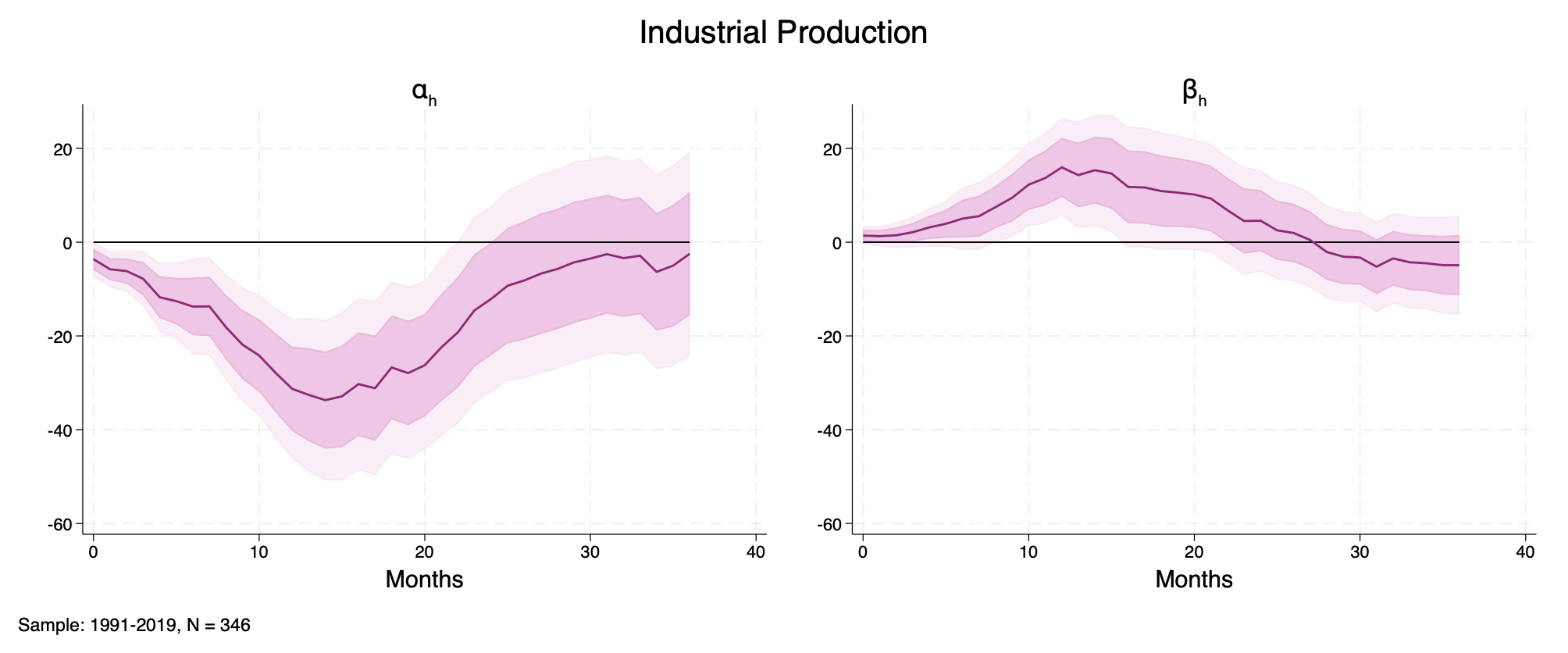
Figure 9. Impulse Response Functions of Industrial Production to an orthogonalized monetary policy shock, estimated from lag-augmented local projections controlling for VIXt and its lags, equation (3). Left panel: αh; right panel: βh. Confidence bands at 68 and 90% levels. Sample: 1991–2019, N = 345 observations (excludes 2001M9 for the 9/11 Terrorist Attacks).
3.3.2 Disagreement and Monetary Surprises
Analyzing how disagreement interacts with monetary policy surprises.
I map lead-lag correlations between shocks and disagreement, re-estimate equation (2) with multiple surprise series, and verify shocks look identical across disagreement states so the documented attenuation reflects heterogeneous transmission rather than differences in the treatment itself.
Another valid concern is the potential causal interplay between the shocks proxy, $s_t$, and the measure of disagreement adopted, $\lvert \overline{D}_t \rvert$ (or $\hat D_t$ for an asymmetric specification, see 3.3.4 below). In fact, even if monetary shocks are exogenous (as suggested by Bauer and Swanson (2023b), Amodeo (2025)), the potential feedback between the policy surprises and the expected FFR paths of Fed and financial markets could hinder the inference drawn on the estimated coefficients (Angrist and Pisckhe (2009)). Intuitively, identification requires the “treatment” – the shock – to be orthogonal to the conditioning state (mathematically, the interacting variable) – disagreement.
I address this by investigating the correlation between the two objects of interest. In particular, a lead-lag correlation map is useful to understand the dynamic relationships between variables over time, allowing for delay or anticipation in the response of one to the other. Figure 10 displays two maps: on the left, the correlation between the baseline orthogonalized $s_t$ and the absolute value of average disagreement $\lvert \overline{D}_{t+\ell} \rvert$, shifted ±12 months; on the right, an alternative specification of the interacting variable without the absolute value, allowing then the full range of motion of the conditioning state in the regressions in (2).
All across the two-year range, the correlation between monetary policy shocks and disagreement is close to zero, and never significant. Appendix D.7 provides a number of alternative comparisons, using a variety of influential surprise series, and details the construction of the 95% confidence bands.
Moreover, I replace the orthogonalized surprises with leading alternative shock series (Gertler and Karadi (2015), Miranda-Agrippino and Ricco (2021), Jarociński and Karadi (2020)), and re-estimate all core specifications. I also estimate the same local projections using the original Bauer and Swanson (2023a) shock series, removing the adjustment in Amodeo (2025). The impulse responses and interaction patterns remain qualitatively unchanged: disagreement still attenuates conventional transmission on output. This stability reduces dependence on any one high-frequency identification technique, mitigates concerns about the orthogonalization treatment, and increases external validity. In sum, the mechanism is robust and economically significant across datasets, samples, and controls.
Finally, another relevant concern is that the attenuation I document might be spurious if the shock itself differs across disagreement states. I address treatment homogeneity in Appendix D.8, proceeding in two steps: first, I estimate the same local projections with the interest rates (FFR, 1-year and 2-year Treasury yields) as outcome variables, including baseline and other influential shock series (D.8.1; D.8.2); second, I explicitly test that the identified shock is distributionally invariant across disagreement quartiles (D.8.3). Although the FFR shows slightly differential effects across disagreement states, these go in the opposite direction as they would to explain the evidence of attenuation (Figure D8), strengthening, if anything, the role of disagreement in transmission; at longer maturities – more relevant and widely used – shocks are comparable across states. Moreover, histograms and densities (Figures D16, D17) and nonparametric tests (Table D1) detect no differences in the conditional distribution of shocks across disagreement quartiles. Overall, the evidence indicates that shocks are statistically indistinguishable across disagreement states (i.e., treatment homogeneity is verified), securing inference and corroborating heterogeneous transmission as the source of attenuation.
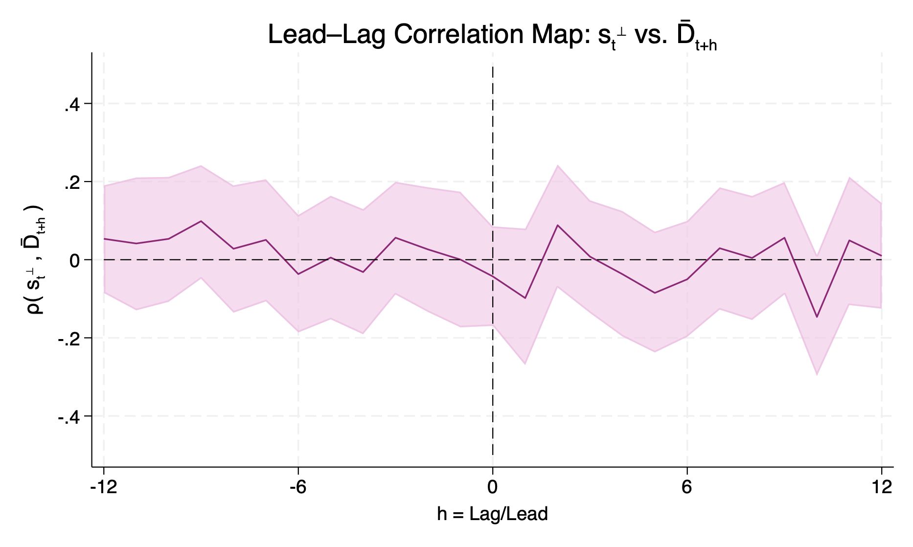
Figure 10. Left panel: Lead-Lag correlation map between orthogonalized monetary policy shocks, and absolute average disagreement. Right panel: Lead-Lag correlation map between orthogonalized monetary policy shocks, and average disagreement. 95% confidence bands computed with Fisher’s z-transform (exact method). Estimation sample: 1990-2019, \(N = 358\) observations (excludes 2001M9 for the 9/11 Terrorist Attacks).
Amodeo (JMP, 2025)
"This paper studies the impact of interest rate disagreement between the Federal Reserve and financial markets on the transmission of U.S. monetary policy. First, I construct a simple real-time measure of disagreement and show that it improves short- and medium-horizon forecasts in standard macroeconomic VARs. Second, using lag-augmented local projections, I show that disagreement dampens monetary policy effectiveness, attenuating its impact on output and offering an explanation for apparent anomalies such as the 'activity puzzle.' Third, I demonstrate that market expectations, as reflected in tradable asset prices, outperform Fed staff forecasts, and that information-advantage tests reveal no systematic Fed edge, challenging prevailing narratives. I show that standard New Keynesian frameworks with incomplete information contain a latent disagreement structure, which, when formalized, yields a parsimonious explanation of the documented evidence. The model generates disagreement from three distinct sources — fundamentals, policy rule, and credibility. A general state-space model identifies the importance of each and sheds light on key normative implications."
B.1 Mechanics of Diebold–Mariano Tests
I have actual data \(\{y_t\}\) and two forecasts \(\{f_{1,t}\}\), \(\{f_{2,t}\}\). For mean-squared-error loss, define the per-forecast errors and their difference:
$$e_{i,t} = (y_t - f_{i,t})^2,\qquad d_t = e_{1,t} - e_{2,t},\qquad \bar d = \frac{1}{T} \sum_{t=1}^{T} d_t$$
Long-run variance:
$$\hat{\gamma}(l) = \frac{1}{T} \sum_{t=l+1}^{T} (d_t - \bar d)(d_{t-l} - \bar d),\qquad \hat{j} = \hat{\gamma}(0) + 2 \sum_{l=1}^{L} w_l \, \hat{\gamma}(l)$$
\(L\) is maxlag (SIC); \(w_l\) depends on kernel (uniform \(w_l = 1\), Bartlett \(w_l = 1 - \tfrac{l}{L+1}\)).
Test statistic:
$$DM = \frac{\bar d}{\sqrt{\hat{j}/T}},\qquad p\text{-value} = 2\big[1 - \Phi(|DM|)\big]$$
where \(\Phi(\cdot)\) is the standard normal CDF.
Null Hypothesis: Equal forecast accuracy; reject if \(p\) is small.
Appendix B: Alternative Timing Assumptions
Tables B1–B2 below report alternative timing assumption in testing comparative accuracy through Diebold-Mariano tests. Respectively, they use as cutoff dates the trading day before the FOMC meeting, and the actual FOMC meeting day. Essentially, this amounts to providing the market with more information, as, on average, the Tealbooks are released internally 6.6 days. Thus, it is unsurprising to see that markets' forecasts confirm their predictive superiority, but I display the results anyway as a sanity check that the procedure works as expected.
Table B1. Diebold–Mariano tests of equal predictive accuracy (Market vs Fed) across horizons with Market's forecast on the day before the FOMC meeting. Reported are sample size \(N\), test statistic, \(p\)-value, and the lower-MSE winner.
Table B2. Diebold–Mariano tests of equal predictive accuracy (Market vs Fed) across horizons with Market's forecast on the day of the FOMC meeting. Reported are sample size \(N\), test statistic, \(p\)-value, and the lower-MSE winner.
C Granger Causality in VAR Forecasting
Idea: determines whether a time series affects the predictions another. If adding it reduces forecast error, we say it Granger-causes the variable
Block-Wise Test: Let \(y_{1,t}\) denote the \(m_1\) "cause" variables and \(y_{2,t}\) denote the \(m_2\) "effect" variables. Consider a stationary VAR(p) model for \([y_{1,t}, y_{2,t}]\):
$$ \begin{bmatrix} y_{1,t} \\ y_{2,t} \end{bmatrix} = c + \delta t + \beta x_t + \begin{bmatrix} \Phi_{11,1} & \Phi_{12,1} \\ \Phi_{21,1} & \Phi_{22,1} \end{bmatrix} \begin{bmatrix} y_{1,t-1} \\ y_{2,t-1} \end{bmatrix} + \cdots + \begin{bmatrix} \Phi_{11,p} & \Phi_{12,p} \\ \Phi_{21,p} & \Phi_{22,p} \end{bmatrix} \begin{bmatrix} y_{1,t-p} \\ y_{2,t-p} \end{bmatrix} + \begin{bmatrix} e_{1,t} \\ e_{2,t} \end{bmatrix} $$
The block-wise Granger causality test hypotheses are:
$$ \begin{aligned} H_{0} &: \Phi_{21,1} = \cdots = \Phi_{21,p} = 0_{m_{2} \times m_{1}} \\ H_{1} &: \exists j \in \{1,\ldots,p\} \text{ s.t. } \Phi_{21,j} \neq 0_{m_{2},m_{1}} \end{aligned} $$
D.7 Lead-Lag Correlation Maps: Details & Extras
This appendix details the procedure used to map the lead-lag relation between the monetary surprise \(s_{t}\) and disagreement \(D_{t}\) over horizons \(h \in [-H, H]\).
Step 1: Shift & correlate. For each \(h \in [-H, H]\) compute
$$\hat{\rho}_{h} = \operatorname{corr}(s_{t}, D_{t+h})$$
where \(D_{t+h} = L^{h} D_{t}\) if \(h > 0\) and \(F^{|h|} D_{t}\) if \(h < 0\). (Here \(L\) and \(F\) denote the one-period lag and lead operators, respectively.)
Step 2: Exact 95% band (Fisher-z).
$$z_{h} = \tfrac{1}{2} \ln\!\left(\frac{1 + \hat{\rho}_{h}}{1 - \hat{\rho}_{h}}\right), \quad \mathrm{SE} = \frac{1}{\sqrt{N - 3}}$$
$$z_{h}^{\pm} = z_{h} \pm 1.96\,\mathrm{SE}, \quad \rho_{h}^{\pm} = \tanh\!\big(z_{h}^{\pm}\big)$$
\(N\) is the number of overlapping \((s_{t}, D_{t+h})\) pairs at horizon \(h\).
Step 3: Plot. Draw \(\hat{\rho}_{h}\) against \(h\) with the shaded confidence band \([\rho_{h}^{-}, \rho_{h}^{+}]\) and dotted axes at \(h = 0\) and \(\rho = 0\).
Interpretation. Values \(\hat{\rho}_{h} > 0\) for \(h > 0\) indicate that disagreement is Granger-predicted by the surprise (information in \(s_{t}\) precedes \(D_{t}\)). Values \(\hat{\rho}_{h} > 0\) for \(h < 0\) indicate that shocks are moved by precedent disagreement.
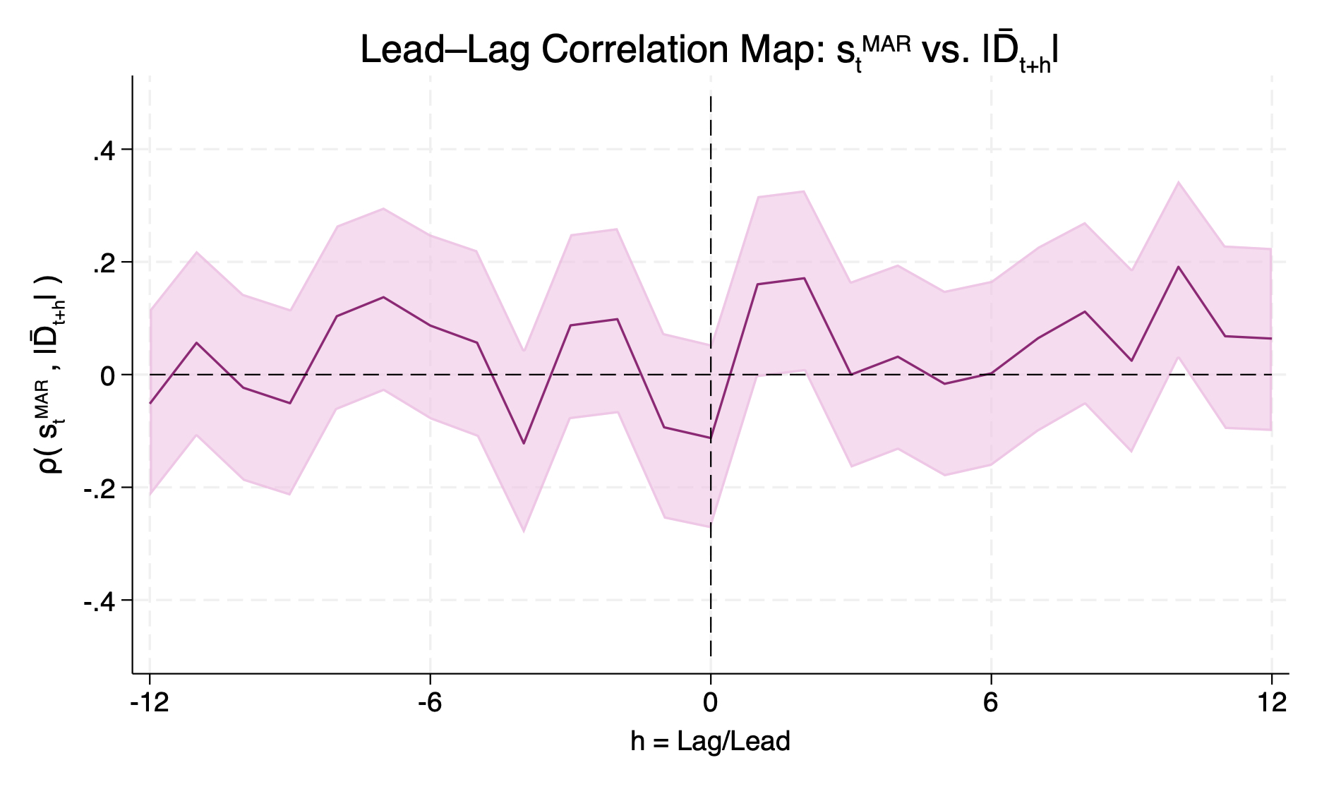
Figure D7.1. Lead-Lag Correlation Map: \(s_{t}^{\mathrm{MAR}}\) vs. \(|\bar{D}_{t+h}|\).
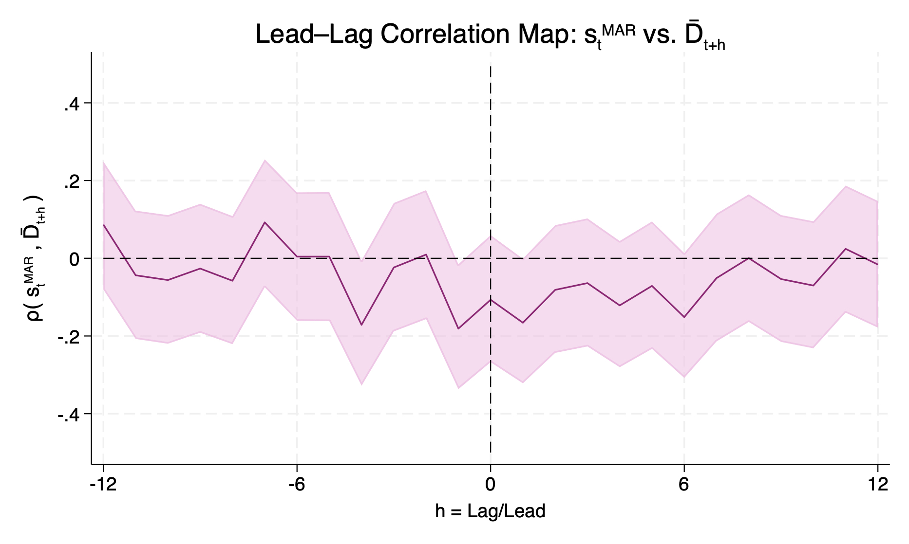
Figure D7.2. Lead-Lag Correlation Map: \(s_{t}^{\mathrm{MAR}}\) vs. \(\bar{D}_{t+h}\).
D.8 Treatment Homogeneity
This appendix tests whether the monetary policy shock differs across disagreement states. I re-estimate the local projections using interest-rate outcomes—the federal funds rate (FFR), 1-year, and 2-year Treasury yields—in a three-variable system and in standard specifications (Gertler and Karadi, 2015, Bauer and Swanson, 2023b). I also replace the orthogonalized surprises with leading alternatives (Gertler and Karadi, 2015, Jarocínski and Karadi, 2020, Miranda-Agrippino and Ricco, 2021). Let \(\alpha_{h}\) denote the IRF in the low-disagreement state and \(\beta_{h}\) the incremental response when \(|D_{t}|\) is high. If \(\beta_{h} \simeq 0\), the identified shock is comparable across states; deviations would indicate state-dependent shocks rather than transmission.
D.8.1 Rate-Outcome Evidence
3-variable SVAR In the differential response depicted in Figure D8, \(\beta_{h}\) is positive and statistically non-negligible at the peak. High-disagreement meetings feature slightly larger policy-rate moves. However, this pattern goes in the opposite direction of what would be needed to mechanically generate attenuation in macro outcomes, and therefore strengthens the heterogeneous-transmission interpretation.
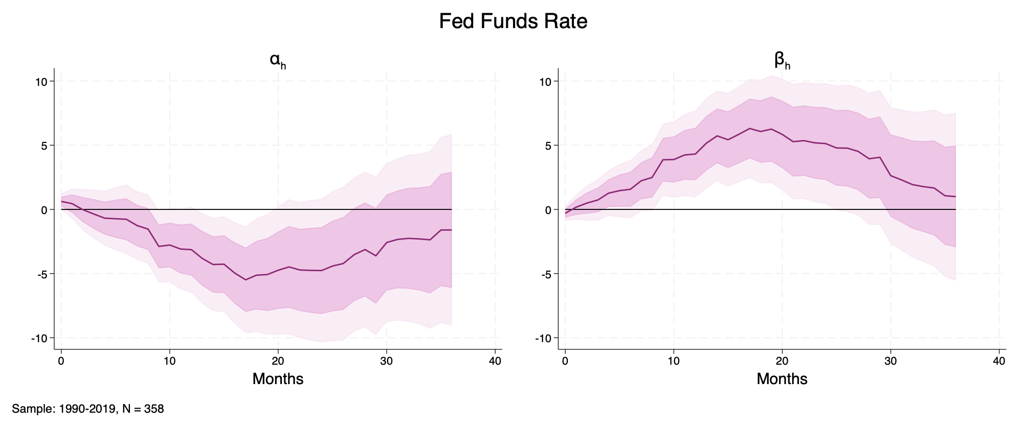
Figure D8. Fed Funds Rate. Local-projection IRFs from the 3-variable system shocked by orthogonalized monetary surprises (Bauer and Swanson (2023a), Amodeo (2025)). Left panel: baseline response \(\alpha_{h}\). Right panel: differential response \(\beta_{h}\). Sample: 1990-2019, \(N = 358\).
Gertler and Karadi (2015)'s SVAR Figure D9. Across the policy-relevant window, \(\beta_{h}\) is close to zero with overlapping bands. Shocks are essentially homogeneous across states at the 1-year maturity.
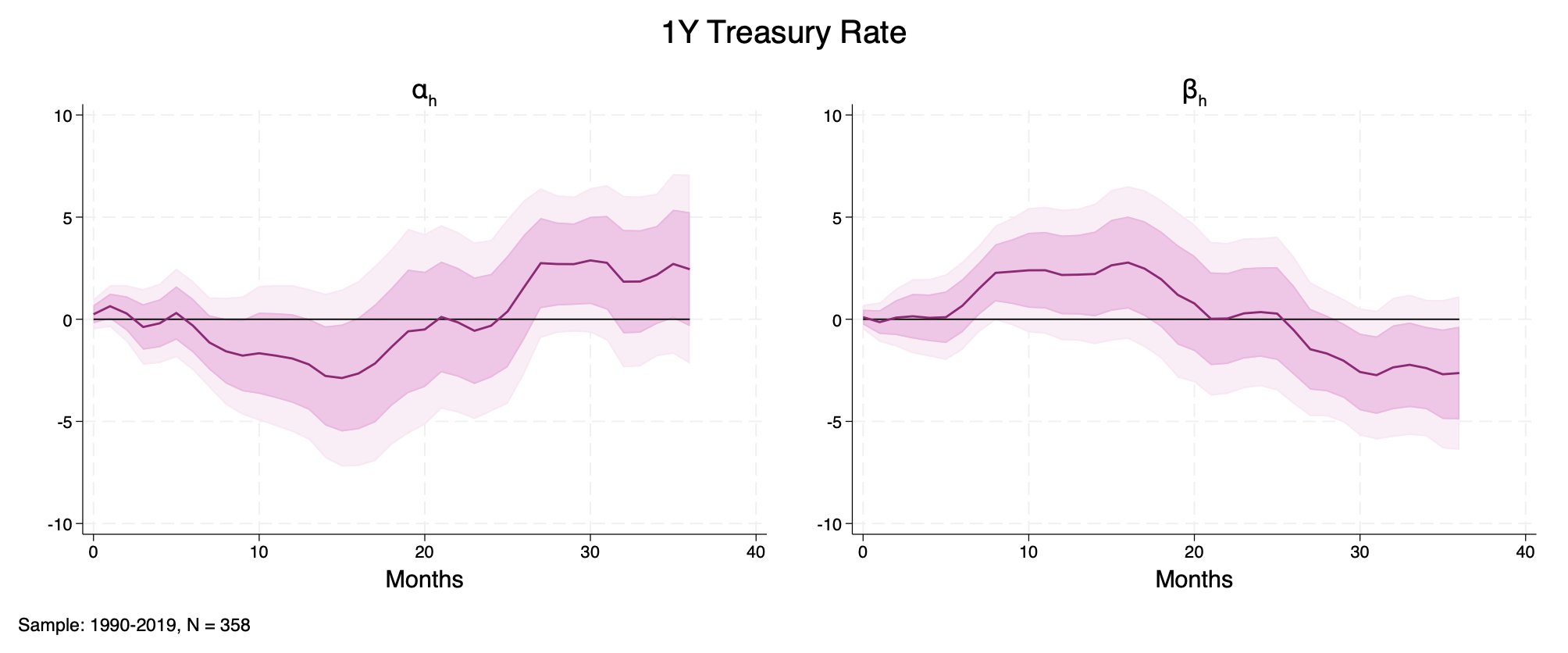
Figure D9. 1-Year Treasury Rate. Local-projection IRFs from the 4-variable system shocked by orthogonalized monetary surprises (Bauer and Swanson (2023a), Amodeo (2025)). Left panel: baseline response \(\alpha_{h}\). Right panel: differential response \(\beta_{h}\). Sample: 1990-2019, \(N = 358\).
Bauer and Swanson (2023b)'s SVAR Figure D.8.1. \(\beta_{h}\) is near zero throughout, and its estimates are less statistically significant than in smaller systems. Shocks appear essentially indistinguishable across states at the 2-year maturity.
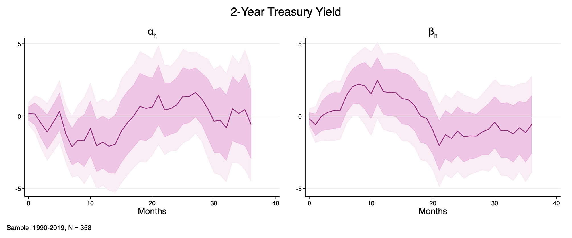
Figure D.8.1. 2-Year Treasury Rate. Local-projection IRFs from the 4-variable system shocked by orthogonalized monetary surprises (Bauer and Swanson (2023a), Amodeo (2025)). Left panel: baseline response \(\alpha_{h}\). Right panel: differential response \(\beta_{h}\). Sample: 1990-2019, \(N = 358\).
D.8.2 Alternative Shocks
This section verifies that results are not driven by the shock measure. For each leading identification, the 3-variable LP with industrial production delivers the same qualitative pattern: \(\alpha_{h}\) shows a contraction followed by recovery, while the \(|D_{t}|\)-dependent effects \(\beta_{h}\) have a similar shape.
Bauer and Swanson (2023b)'s original shock Unadjusted orthogonalized monetary surprise.
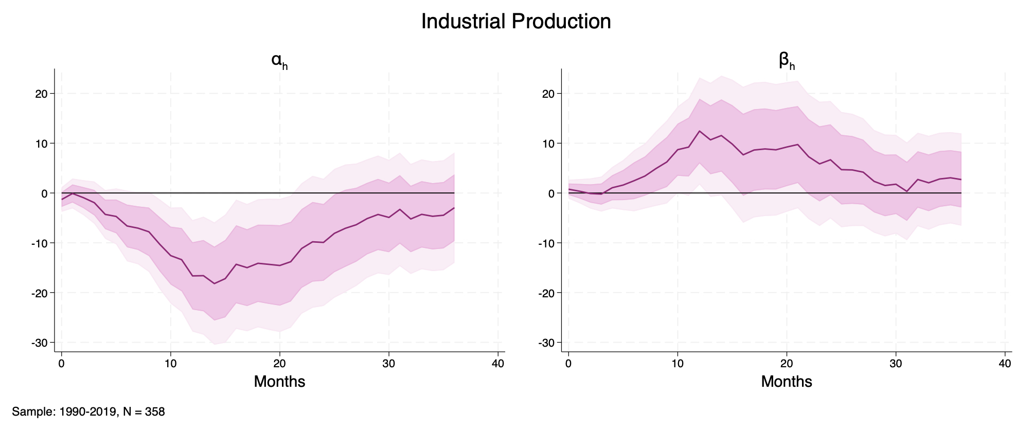
Figure D11: Industrial Production, 3-variable system shocked by orthogonalized monetary surprises as in Bauer and Swanson (2023b). Left: \(\alpha_{h}\); Right: \(\beta_{h}\). Sample: 1990–2019, \(N = 358\).
Gertler and Karadi (2015)'s shock
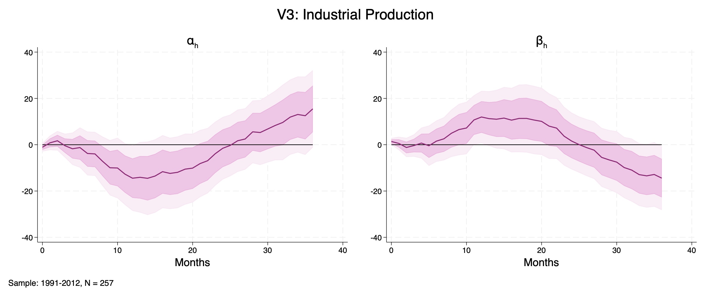
Figure D12: Industrial Production. 3-variable system shocked by high-frequency monetary surprises as in Gertler and Karadi (2015). Left: \(\alpha_{h}\); Right: \(\beta_{h}\). Sample: 1991–2012, \(N = 257\).
Miranda-Agrippino and Ricco (2021)'s MPI shock
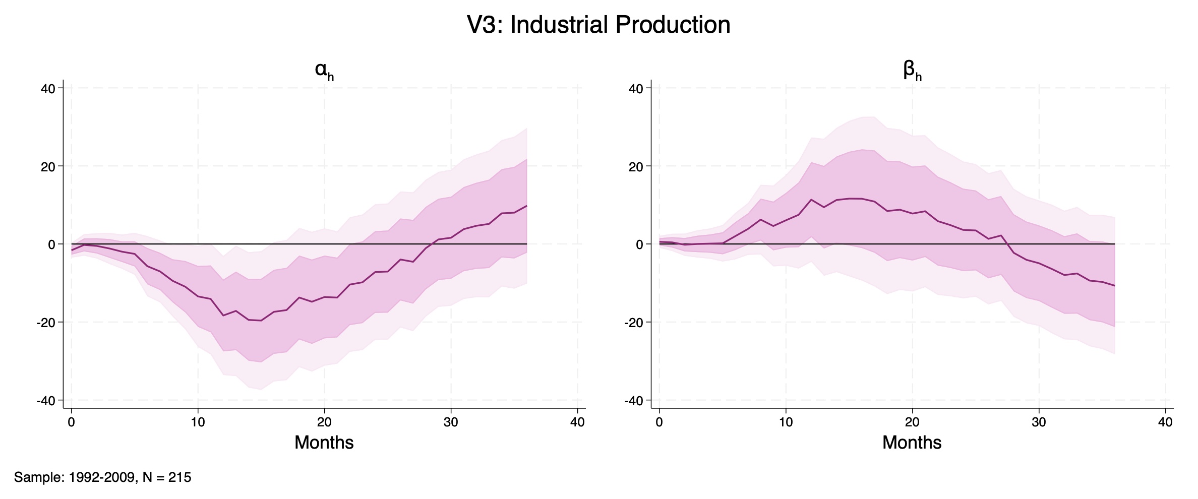
Figure D13: Industrial Production, 3-variable system shocked by high-frequency Monetary Policy Instrument (MPI) as in Miranda-Agrippino and Ricco (2021). Left: \(\alpha_{h}\); Right: \(\beta_{h}\). Sample: 1992–2009, \(N = 215\).
Jarociński and Karadi (2020)'s First Principal Component shock
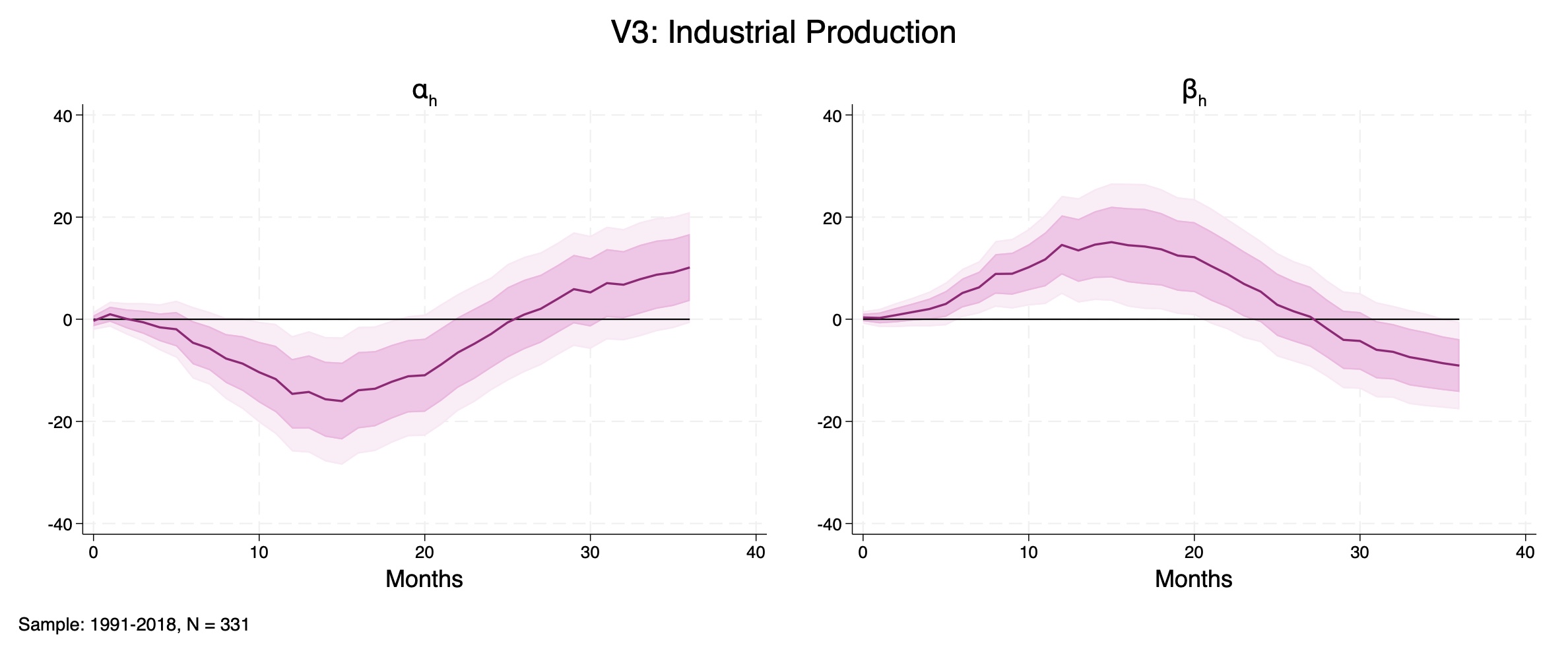
Figure D14: Industrial Production, 3-variable system shocked by high-frequency monetary surprises as in Jarociński and Karadi (2020) (first principal component). Left: \(\alpha_{h}\); Right: \(\beta_{h}\). Sample: 1991–2018, \(N = 331\).
Jarociński and Karadi (2020)'s Identified Monetary Policy shock
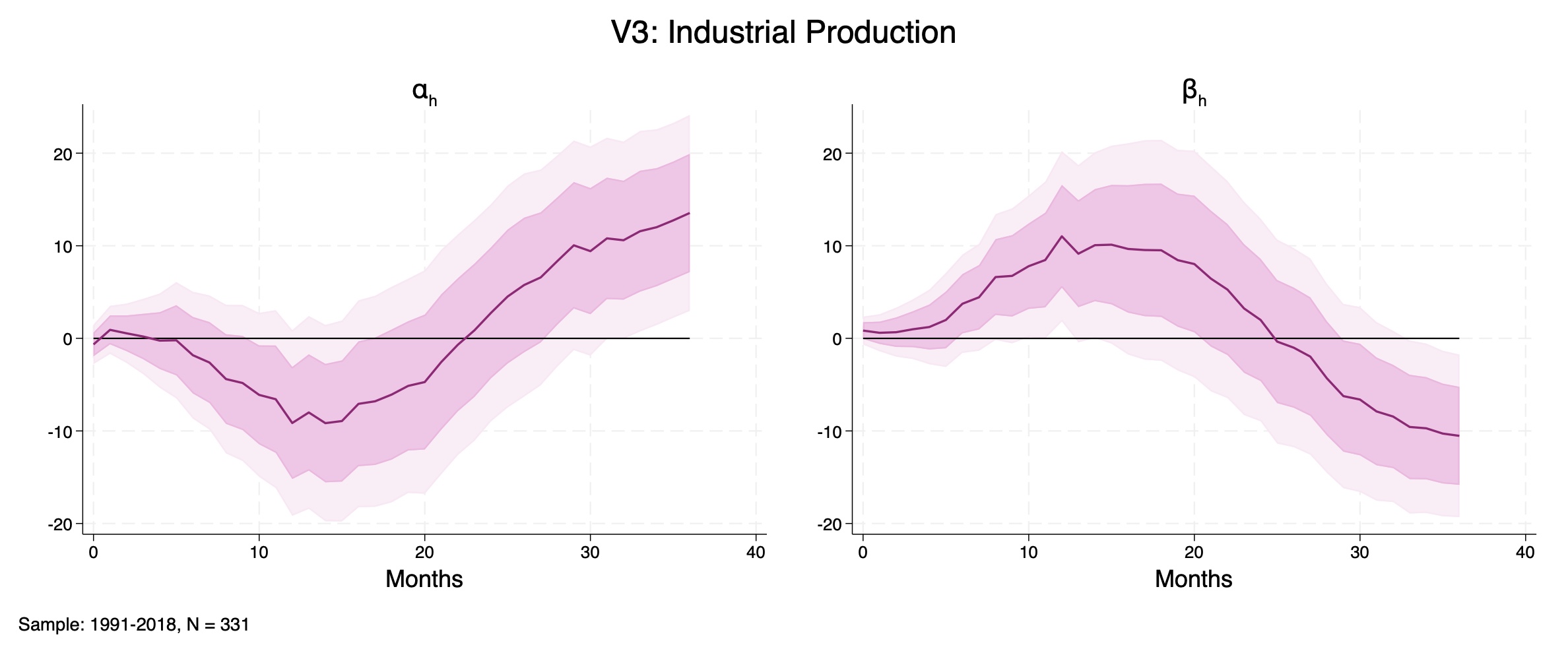
Figure D15: Industrial Production, 3-variable system shocked by high-frequency monetary surprises as in Jarociński and Karadi (2020) (monetary shock "poor man" version). Left: \(\alpha_{h}\); Right: \(\beta_{h}\). Sample: 1991–2018, \(N = 331\).
D.8.3 Shocks Across Disagreement States
This appendix tests whether the monetary shock is drawn from the same distribution across quartiles of absolute average Fed–Market disagreement \(|\bar{D}_{t}|\). Causal claims about state-dependent transmission require treatment homogeneity: if the shock’s distribution changes with the state, estimated heterogeneity could reflect different treatments rather than different propagation.
Results reveal that disagreement states do not conceal distinct shock regimes. Then, it is unlikely for the results to be driven by the shocks themselves differing across states, supporting the paper’s main point of differential policy transmission.
Figure D16 shows the histograms of the baseline shocks across quartiles of the interacting variable (absolute average disagreement). The four panels look similar: centered at zero with the same sharp spike at 0, thin and broadly symmetric tails, and no visible shift in mass across quartiles. Because bins and axes are kept identical, visual similarity is meaningful. Moreover, I next implement statistical formal tests of distributional similarity. Figure D17 displays the same notions in a more direct way using kernel densities.
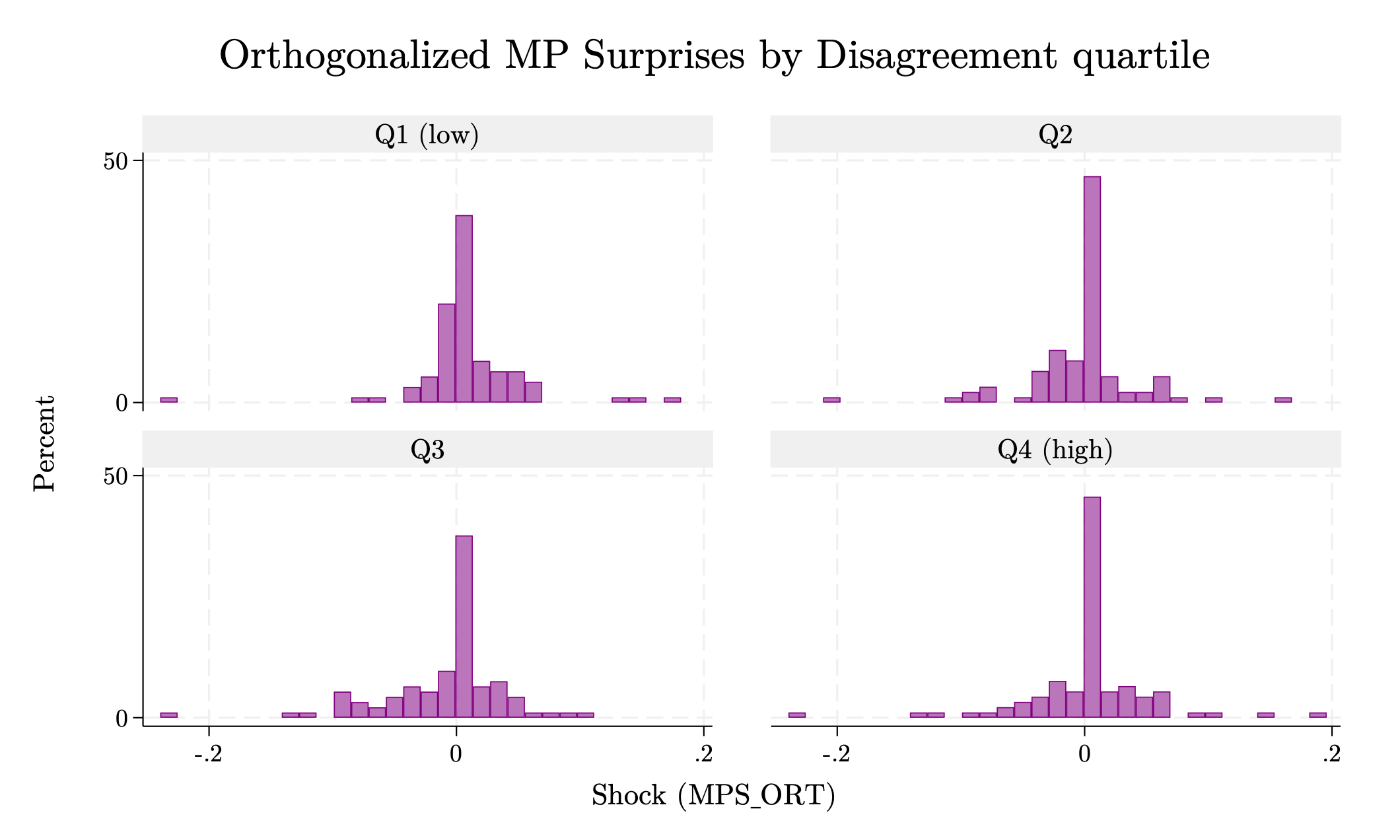
Figure D16: Histograms of \(s_{t}\) by disagreement quartile; percent scale.
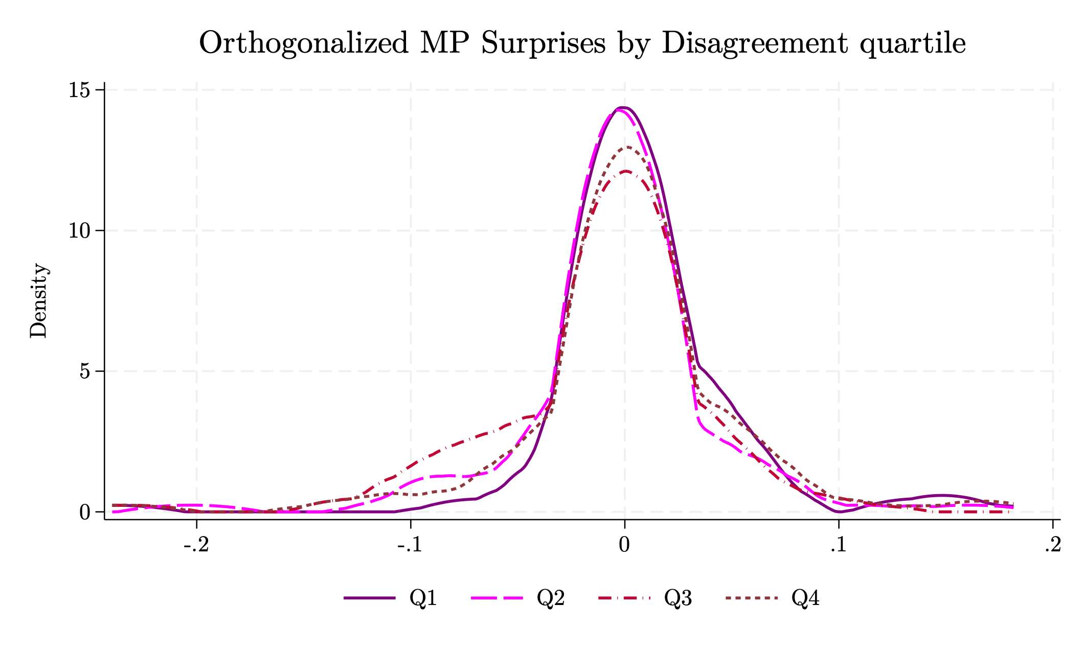
Figure D17: Kernel densities of \(s_{t}\) by disagreement quartile. A single bandwidth is used for all groups and the support is held fixed.
Table D1 displays analytical results from the comparison of shocks across disagreement quartiles. Means are near zero in every quartile; standard deviations rise modestly with disagreement, consistent with mild heteroskedasticity. The mass at zero is statistically identical across groups.
Panel A reports sample size, means, dispersion (SD), and the share of exact zeros by quartile. Panel B reports \(p\)-values from nonparametric tests: equality of typical levels (Kruskal–Wallis), equality of zero shares, and pairwise KS tests of whole-distribution equality. When \(p > 0.05\) we treat groups as statistically similar for that feature.
Kruskal–Wallis asks whether the typical level of the shock is the same across groups without assuming normality. The “zero-mass” test simply compares the share of exact zeros across groups. The two-sample Kolmogorov–Smirnov (KS) test compares the entire shape of two distributions—center, spread, and tails—at once. Large \(p\)-values in these tests mean the data do not provide evidence of differences across disagreement states.
Kruskal–Wallis tests fail to reject equal locations. The proportion of zeros is constant as well. Finally, only one unadjusted KS comparison is low (Q1–Q3), but it is not significant after Holm–Bonferroni across six pairs. In summary, graphical inspection and formal tests allow us to treat shocks as distributionally equivalent across disagreement states.
Panel A. Moments by quartile.
| Q1 (low) | Q2 | Q3 | Q4 (high) | |
|---|---|---|---|---|
| \(N\) | 93 | 92 | 93 | 92 |
| Mean | 0.0069 | -0.0030 | -0.0105 | 0.0018 |
| SD | 0.0440 | 0.0435 | 0.0478 | 0.0515 |
| \(\Pr(s_{t} = 0)\) | 0.269 | 0.326 | 0.333 | 0.304 |
Panel B. Distributional tests (\(p\)-values unless noted).
| Test | Statistic | \(p\)-value |
|---|---|---|
| Kruskal–Wallis \(\chi^{2}(3)\) | 6.355 | 0.0956 |
| Zero-mass test \(\chi^{2}(3)\) | 1.097 | 0.7778 |
Two-sample Kolmogorov–Smirnov \(p\)-values.
| Q1 | Q2 | Q3 | Q4 | |
|---|---|---|---|---|
| Q1 | — | 0.304 | 0.027 | 0.519 |
| Q2 | 0.304 | — | 0.551 | 0.771 |
| Q3 | 0.027 | 0.551 | — | 0.291 |
| Q4 | 0.519 | 0.771 | 0.291 | — |
Table D1. Moments and distributional tests of \(s_{t}\) across disagreement quartiles. Quartiles by \(|\bar{D}_{t}|\). KS entries are combined \(p\)-values. After family-wise error control (Holm–Bonferroni), no KS comparison is significant at 5%.
To quantify gains, I use the partial \(R^{2}\) for nested models:
This measures the percent drop in unexplained variance.
Similarly, average disagreement exhibits an even more negative correlation.
For reasons of length and flow, I include (i) in the body, and defer (ii) to Appendix D.5.
I include all the lag-terms in a generally defined $\text{Lags}_{t-1}^L$ term. This comprises the lags of both dependent and control variables, and the lags of the shocks and interacted variables.
Single calendar year averages are depicted in Figure B1, Appendix B, and horizon‑specific comparisons display similarly inconclusive insights.
Appendix B also includes comparisons with the Survey of Professional Forecasters’ consensus—whose timing is inherently coarser—yield similar rank‑fluctuation patterns.
Distinct, conceptually, from information advantage tests, which ask whether one forecast adds information conditional on the other: it can be shown that such tests do not rank forecast accuracy unless both forecasts are unbiased and their errors uncorrelated. With correlation or bias, the mapping breaks. Giacomini and Rossi (2010), instead, targets accuracy directly by tracking the mean loss differential, regardless of the correlation structure.
Technical specifications are reported in Appendix D.10.
For instance, I replicate the test not only timing markets’ forecast to the Tealbook cutoff date, but also experiment with one and three days in advance futures prices, to allow a buffer in case the Tealbook predictions were formulated before their release date. Appendix D.10.1 reports the additional results.
Let \(\widehat{V}_{t}\) be the Newey–West estimate of the long‑run variance matrix \(V\) in the \(m\)-observation window at time \(t\). Define
Critical values are the two‑sided t‑statistics analogous to the Wald test values for the survey and model‑free forecasts reported in Table II, Panel C of Rossi and Sekhposyan (2016), resimulated to match the sample size and rolling window length.
A rejection rules out the hypothesis that the central bank never had an information advantage. Previous studies using surveys report an evident advantage; by contrast, these results contradict that view, as the statistic crosses the critical bands only episodically.
In Appendix D.10, I report results for a variety of window lengths and window/sample ratios, including the \(m = 60\) specification Hoesch et al. (2023) implement, to facilitate a like‑for‑like comparison.
Simplified Notation. The full specification can be written more compactly as:
where the lag block collects all lagged regressors:
with respective coefficients: